Univariate examples

Installation

library(predRecruit)
library(ggplot2)

Parametric and semi-parametric examples

We can fit linear regression and generalized additive models using the univariate() function. Here, we’ll simulate some dummy data. Our response has 40 time steps, and the matrix of predictors includes 4 potential covariates.

response <- data.frame(time = 1:40, dev = rnorm(40))

predictors <- matrix(rnorm(4 * 40), ncol = 4)
#' #colnames(predictors) = paste0("X",1:ncol(predictors))
predictors <- as.data.frame(predictors)
predictors$time <- 1:40
lm_example <- univariate_forecast(response,
  predictors,
  model_type = "lm", # can be 'lm' or 'gam'
  n_forecast = 10, # how many years of data to use in testing
  n_years_ahead = 1, # how many time steps ahead to forecast
  max_vars = 3) # maximum number of covars allowed in any one model

The returned object is a list with 4 elements

names(lm_example)

## [1] "pred"     "vars"     "coefs"    "marginal"

These elements are * pred, a dataframe consisting of our original data, with responses and covariates binded together. Also includes model predictions est, uncertainty se and several metrics describing the fit to the training data (train_r2 and train_rmse). * vars, a dataframe containing the combination of each unique set of covariates included, ranging from 1 to max_vars * coefs, a list containing coefficients elements for each model that was fit. For models with n_forecast larger than 1, a set of coefficients will be returned for each year that is used as a holdout datapoint. For the above example, we can look at

lm_example$coefs[[1]]

## # A tibble: 30 × 6
##    term  estimate std.error statistic p.value    yr
##    <chr>    <dbl>     <dbl>     <dbl>   <dbl> <int>
##  1 cov1   0.0590      0.205    0.287    0.776    31
##  2 cov2  -0.244       0.237   -1.03     0.313    31
##  3 cov3   0.00299     0.187    0.0160   0.987    31
##  4 cov1   0.0441      0.209    0.211    0.834    32
##  5 cov2  -0.160       0.234   -0.684    0.500    32
##  6 cov3  -0.0352      0.188   -0.187    0.853    32
##  7 cov1   0.0397      0.202    0.196    0.846    33
##  8 cov2  -0.149       0.214   -0.697    0.491    33
##  9 cov3  -0.0276      0.175   -0.157    0.876    33
## 10 cov1   0.0302      0.193    0.156    0.877    34
## # … with 20 more rows

and see that there are 10 sets of the 3 coefficients, along with standard errors and p-values for each (yr ranging from 31 to 40).

marginal, also a list with each element specific to a specific model this contains the marginal effects of each parameter and can be useful in identifying non-linear relationships with GAMs.

Using the above example output, we can plot the marginal effects for the first model,

marg <- lm_example$marginal[[1]]

# focus on the marginal effects for the full dataset
marg <- dplyr::filter(marg, year == max(marg$year))

ggplot(marg, aes(x, predicted)) + 
  geom_ribbon(aes(ymin=conf.low, ymax = conf.high)) + 
  geom_line() + 
  facet_wrap(~cov, scale="free", nrow=2) + 
  ylab("Marginal effect") + 
  xlab("Covariate")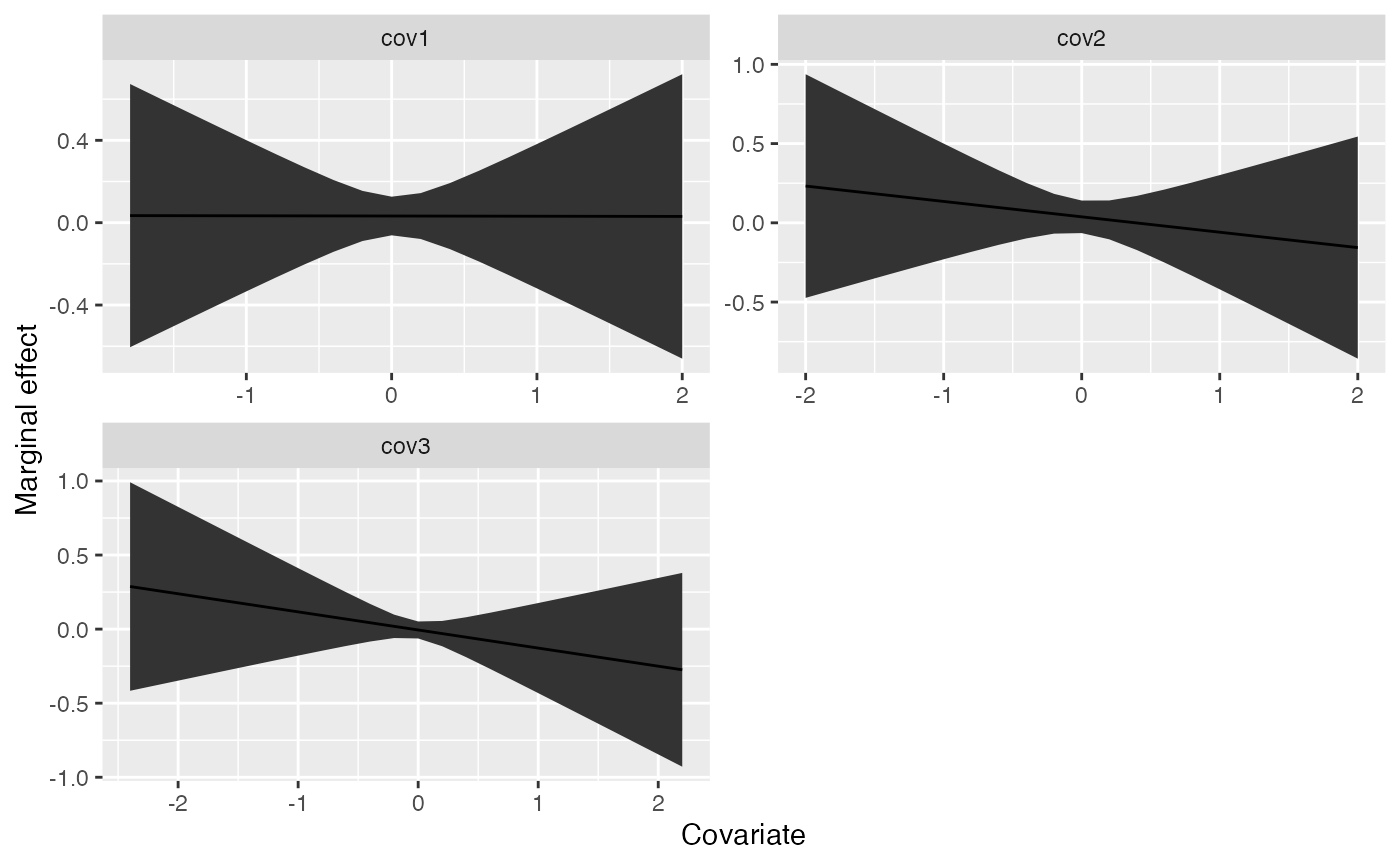

Non-parametric examples

Using our above dummy dataset, we can also try to use random forest or lasso / ridge regression methods to generate forecasts. These are done with the univariate_forecast_ml function.

lm_example <- univariate_forecast_ml(response,
    predictors,
    model_type = "glmnet", # can be "glmnet" or "randomForest"
    n_forecast = 10,
    n_years_ahead = 1)

The main difference between the parametric or semi-parametric approaches and the non-parametric ones are that we are not generating marginal effects. Similarly, the fitted object is slightly different – this only includes 2 elements, * pred, a dataframe containing the original data (responses and predictors) along with estimated deviations * tuning, a dataframe containing the tuning parameters that were explored for each row (id)

Eric Ward

2023-01-19

Installation

Parametric and semi-parametric examples

Non-parametric examples